Das Vektorprodukt

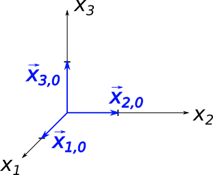
Das kartesische Koordinatensystem ist so aufgebaut, dass das Vektorprodukt der $x_1$-Achse mit der $x_2$-Achse genau die $x_3$-Achse ergibt. Es gilt also: $$ \vec x_1 \times \vec x_2 = \vec x_3 $$ In diesem Sinne kann auch die Vektormultiplikation der Einheitsvektoren der Koordinatenachsen aufgefasst werden: $$ \vec x_{1,0} \times \vec x_{2,0} = \vec x_{3,0} $$ Wichtig ist hier vor allem die Reihenfolge. Mit der rechten Hand-Regel kann man sich die Reihenfolge klar machen. Der Daumen zeigt in die $x_1$-Richtung, der Zeigefinger in die $x_2$-Richtung und der Mittelfinger in die $x_3$-Richtung. Zwischen den Fingern befindet sich jeweils ein rechter Winkel.
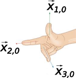Die Reihenfolge ist immer Daumen - Zeigefinger - Mittelfinger - Daumen - Zeigefin... und immer so weiter. Es ist egal, wo man anfängt. Man erhält also z.B. die folgenden Vektorprodukte: \begin{align} \vec x_{1,0} \times \vec x_{2,0} &= \vec x_{3,0} \\ \\ \vec x_{2,0} \times \vec x_{3,0} &= \vec x_{1,0} \\ \\ \vec x_{3,0} \times \vec x_{1,0} &= \vec x_{2,0} \end{align} Es gelten weiterhin die folgenden Zusammenhänge: \begin{align} \vec x_{1,0} \times \vec x_{1,0} = \vec x_{2,0} \times \vec x_{2,0} = \vec x_{3,0} \times \vec x_{3,0} = 0 \end{align}

\begin{align} \vec x_{1,0} \times \vec x_{2,0} = - \left( \vec x_{2,0} \times \vec x_{1,0} \right) &= \vec x_{3,0} \\ \\ \vec x_{3,0} \times \vec x_{1,0} = - \left( \vec x_{1,0} \times \vec x_{3,0} \right) &= \vec x_{2,0} \\ \\ \vec x_{2,0} \times \vec x_{3,0} = - \left( \vec x_{3,0} \times \vec x_{2,0} \right) &= \vec x_{1,0} \\ \\ \end{align}

Zwei weitere Rechengesetze sind: \begin{align} \vec a \times \left( \vec b + \vec c \right) &= \vec a \times \vec b + \vec a \times \vec c \\ \\ \left( r \cdot \vec a \right) \times \vec b &= r \cdot \left( \vec a \times \vec b \right) \end{align}

Herleitung der Berechnungsvorschrift

Zerlegt man die beiden Vektoren $\vec a$ und $\vec b$ in ihre Bestandteile, insbesondere mit den Richtungseinheitsvektoren, erhält man: \begin{align} \vec a &= a_1 \cdot \vec x_{1,0} + a_2 \cdot \vec x_{2,0} + a_3 \cdot \vec x_{3,0} \\ \\ \vec b &= b_1 \cdot \vec x_{1,0} + b_2 \cdot \vec x_{2,0} + b_3 \cdot \vec x_{3,0} \end{align}

Für das Vektorprodukt $\vec a \times \vec b$ ergibt sich zunächst, wenn der Vektor $\vec b$ durch den obigen Ausdruck ersetzt wird: \begin{align} \vec a \times \vec b = \vec a \times \left( b_1 \cdot \vec x_{1,0} + b_2 \cdot \vec x_{2,0} + b_3 \cdot \vec x_{3,0} \right) \end{align} Mit dem ersten der angegebenen Rechengesetze wird das zu: \begin{align} = \vec a \times b_1 \cdot \vec x_{1,0} + \vec a \times b_2 \cdot \vec x_{2,0} + \vec a \times b_3 \cdot \vec x_{3,0} \end{align} Wird der Vektor $\vec a$ in der zerlegten Form in den Ausdruck eingesetzt, folgt: \begin{align} = \left( a_1 \cdot \vec x_{1,0} + a_2 \cdot \vec x_{2,0} + a_3 \cdot \vec x_{3,0} \right) \times b_1 \cdot \vec x_{1,0} \\ + \left( a_1 \cdot \vec x_{1,0} + a_2 \cdot \vec x_{2,0} + a_3 \cdot \vec x_{3,0} \right) \times b_2 \cdot \vec x_{2,0} \\ + \left( a_1 \cdot \vec x_{1,0} + a_2 \cdot \vec x_{2,0} + a_3 \cdot \vec x_{3,0} \right) \times b_3 \cdot \vec x_{3,0} \end{align} Mit dem ersten Rechengesetz ergibt sich: \begin{align} = a_1 \cdot \vec x_{1,0} \times b_1 \cdot \vec x_{1,0} + a_2 \cdot \vec x_{2,0} \times b_1 \cdot \vec x_{1,0} + a_3 \cdot \vec x_{3,0} \times b_1 \cdot \vec x_{1,0} \\ + a_1 \cdot \vec x_{1,0} \times b_2 \cdot \vec x_{2,0} + a_2 \cdot \vec x_{2,0} \times b_2 \cdot \vec x_{2,0} + a_3 \cdot \vec x_{3,0} \times b_2 \cdot \vec x_{2,0} \\ + a_1 \cdot \vec x_{1,0} \times b_3 \cdot \vec x_{3,0} + a_2 \cdot \vec x_{2,0} \times b_3 \cdot \vec x_{3,0} + a_3 \cdot \vec x_{3,0} \times b_3 \cdot \vec x_{3,0} \end{align} Wird das zweite Rechengesetz angewendet, folgt: \begin{align} = a_1 \cdot b_1 \left(\vec x_{1,0} \times \vec x_{1,0} \right) + a_2 \cdot b_1 \left(\vec x_{2,0} \times \vec x_{1,0} \right) + a_3 \cdot b_1 \left(\vec x_{3,0} \times \vec x_{1,0} \right) \\ + a_1 \cdot b_2 \left(\vec x_{1,0} \times \vec x_{2,0} \right) + a_2 \cdot b_2 \left(\vec x_{2,0} \times \vec x_{2,0} \right) + a_3 \cdot b_2 \left(\vec x_{3,0} \times \vec x_{2,0} \right) \\ + a_1 \cdot b_3 \left(\vec x_{1,0} \times \vec x_{3,0} \right) + a_2 \cdot b_3 \left(\vec x_{2,0} \times \vec x_{3,0} \right) + a_3 \cdot b_3 \left(\vec x_{3,0} \times \vec x_{3,0} \right) \end{align} Mit den oben angegebenen Zusammenhängen zwischen den Richtungseinheitsvektoren folgt: \begin{align} = 0 + a_2 \cdot b_1 \left(- \vec x_{3,0} \right) + a_3 \cdot b_1 \left(\vec x_{2,0} \right) \\ + a_1 \cdot b_2 \left(\vec x_{3,0} \right) + 0 + a_3 \cdot b_2 \left(- \vec x_{1,0} \right) \\ + a_1 \cdot b_3 \left(- \vec x_{2,0} \right) + a_2 \cdot b_3 \left(\vec x_{1,0} \right) + 0 \end{align} Sortiert man das nach den Einheitsvektoren, bekommt man: \begin{align} = a_2 \cdot b_3 \left(\vec x_{1,0} \right) - a_3 \cdot b_2 \left(\vec x_{1,0} \right) \\ + a_3 \cdot b_1 \left(\vec x_{2,0} \right) - a_1 \cdot b_3 \left(\vec x_{2,0} \right) \\ + a_1 \cdot b_2 \left(\vec x_{3,0} \right) - a_2 \cdot b_1 \left(\vec x_{3,0} \right) \end{align} Insgesamt folgt für das Vektorprodukt die folgende Berechnungsvorschrift: \begin{align} \vec a \times \vec b = \left( \begin{array}{} a_2 \cdot b_3 - a_3 \cdot b_2 \\ a_3 \cdot b_1 - a_1 \cdot b_3 \\ a_1 \cdot b_2 - a_2 \cdot b_1 \end{array} \right) \end{align}

Anwendungen

Vektorprodukt

Die zwei Vektoren $\vec a$ und $\vec b$ bilden zwei Seiten eines Parallelogramms. Der Betrag des Vektorprodukts $ \lvert \vec a \times \vec b \rvert$ entspricht dem Flächeninhalt des Parallelogramms.

Beispiel:

Ein Parallelogramm wird durch die beiden Vektoren $\vec a = \left( \begin{array}{} 0 \\ 3 \\ 0 \end{array} \right)$ und $\vec b = \left( \begin{array}{} 2 \\ 1 \\ 0 \end{array} \right)$ aufgespannt.
Das Vektorprodukt ergibt: \begin{align} \left( \begin{array}{} 0 \\ 3 \\ 0 \end{array} \right) \times \left( \begin{array}{} 2 \\ 1 \\ 0 \end{array} \right) = \left( \begin{array}{} 0 \\ 0 \\ -6 \end{array} \right) \end{align} Der Betrag des Vektorprodukts ist dann: \begin{align} \lvert \vec a \times \vec b \rvert = 6 \end{align} Der Flächeninhalt des Parallelogramms ist damit 6 FE.

Spatprodukt

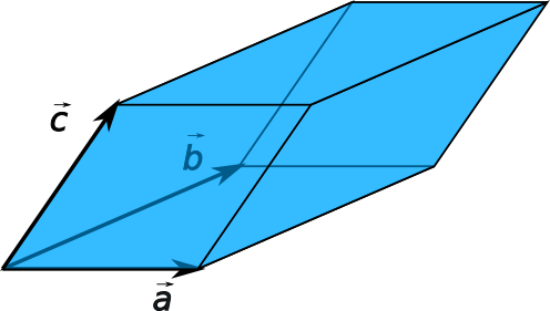Ein Parallelepiped ist ein Körper, der aus sechs paarweise parallelen Parallelogrammen zusammengesetzt wird.

Für die Bestimmung des Volumens eines Parallelepipeds ist das Spatprodukt geeignet. Hier werden Vektor- und Skalarprodukt genutzt.
Man kann für das Spatprodukt aus den drei Vektoren $\vec a$, $\vec b$ und $\vec c$ schreiben: \begin{align} \left( \vec a , \vec b , \vec c \right) = \left( \vec a \times \vec b \right) \cdot \vec c \end{align} Der Betrag des Ergebnisses ist das Volumen des Epipeds.

Beispiel:

Gegeben sind die Vektoren $\vec a = \left( \begin{array}{} -2 \\ 3 \\ 0 \end{array} \right)$, $\vec b = \left( \begin{array}{} 1 \\ 2 \\ -1 \end{array} \right)$ und $\vec c = \left( \begin{array}{} -3 \\ 1 \\ 3 \end{array} \right)$, wie sie in der Abbildung zu sehen sind.

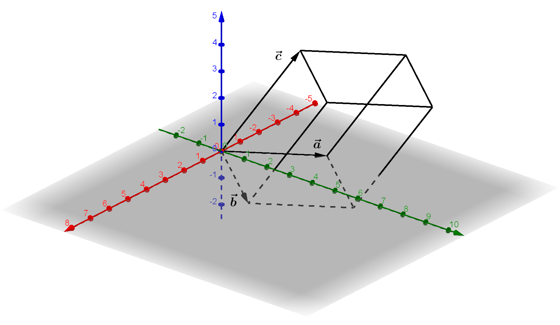
Für das Spatprodukt erhält man: \begin{align} \left( \vec a , \vec b , \vec c \right) &= \left( \left( \begin{array}{} -2 \\ 3 \\ 0 \end{array} \right) \times \left( \begin{array}{} 1 \\ 2 \\ -1 \end{array} \right) \right) \cdot \left( \begin{array}{} -3 \\ 1 \\ 3 \end{array} \right) \\ \\ \left( \vec a , \vec b , \vec c \right) &= \left(\begin{array}{} 3 \cdot (-1) - 2 \cdot 0 \\ 0 \cdot 1 - (-1) \cdot (-2) \\ (-2) \cdot 2 - 1 \cdot 3 \end{array} \right) \cdot \left( \begin{array}{} -3 \\ 1 \\ 3 \end{array} \right) \\ \\ \left( \vec a , \vec b , \vec c \right) &= \left(\begin{array}{} -3 \\ -2 \\ -7 \end{array} \right) \cdot \left( \begin{array}{} -3 \\ 1 \\ 3 \end{array} \right) \\ \\ \left( \vec a , \vec b , \vec c \right) &= (-3) \cdot (-3) + (-2) \cdot 1 + (-7) \cdot 3 \\ \\ \left( \vec a , \vec b , \vec c \right) &= -14 \end{align} Das Volumen ist also $V = 14 \, \text{VE}$.